tl;dr: vanilla residual networks are very good approximators of functions which can be represented as linear perturbations of the identity. In the linear setting, optimization is aided by a benevolent landscape having only minima in certain (interesting) regions. Finally, very simple ResNets can completely learn datasets with $\mathcal{O} (n \log n + \ldots)$ parameters. All this seems to indicate that deep and simple architectures might be enough to achieve great performance.
In general, it is hard for classical deep nets to “preserve features which are good”: initialization with zero mean and small gradients make it hard to learn the identity at any given layer. Even though batchnorm1 seeks to alleviate this issue, it has been residual networks which have most improved upon it.2 In a residual net
(…) each residual layer has the form $x + h (x)$, rather than $h (x)$. This simple reparameterization allows for much deeper architectures largely avoiding the problem of vanishing (or exploding) gradients.
Identity parametrizations improve optimization
The authors work first in the linear setting, i.e. they consider only networks which are compositions of linear perturbations of the identity:3
\[ h (x) = (I + A_{l}) \cdots (I + A_{2}) (I + A_{1}) x \]
The objective function to mimize is the population risk with quadratic loss:
\[ f (A) = f (A_{1}, \ldots, A_{l}) := \mathbb{E}_{X, Y} | Y - (I + A_{l}) \cdots (I + A_{1}) X |^2 . \]
Labels are assigned with noise, that is $Y = RX + \xi$, with $\xi \sim \mathcal{N} (0, I_{d})$. Note that the problem over the variables $A = (A_{1}, \ldots, A_{l})$ is non-convex.
The first result of the paper states that deep networks with many layers have minima of proportionally low (spectral) norm.4 Because of this, it makes sense to study critical points with small norm, and it turns out that there are only minima. The main result of this section is the following one, where one can think of $\tau$ as being $\mathcal{O} (1 / l)$:
Theorem 1: For every $\tau < 1$, every critical point $A$ of the objective function $f$ with \[ \underset{1 \leqslant i \leqslant l}{\max} | A_{i} | \leqslant \tau \] is a global minimum.
This is good news since, under the assumption that the model is correct, a “good” (in some sense) optimization algorithm will converge to it.5 The proof is relatively straightforward too: rewrite the risk as the norm of a product by the covariance: $f (A) = | E (A) \Sigma^{1 / 2} |^2 + C$, then, using that $| A_{i} |$ are small, show that if $\nabla f (A) = 0$ this can only be if $E (A) = 0$, where $E$ precisely encodes the condition of being at an optimum: $E (A) = (I + A_{l}) \cdots (I + A_{1}) - R$.
Identity parametrizations improve representation
The authors consider next non-linear simplified residual networks with each layer of the form
\begin{equation} \label{eq:residual-unit}\tag{1} h_{j} (x) = x + V_{j} \sigma (U_{j} x + b_{j}) \end{equation}
where $V_{j}, U_{j} \in \mathbb{R}^{k \times k}$ are weight matrices, $b_{j} \in \mathbb{R}^k$ is a bias vector and $\sigma (z) = \max (0, z)$ is a ReLU activation.6 Note that the layer size is constant. No batchnorm is applied. The problem is $r$-class classification. Assuming (the admittedly natural condition) that all the training data are uniformly separated by a minimal distance $\rho > 0$, they prove that perfectly learning $n$ data points is possible with $n \log n$ parameters:
Theorem 2: There exists a residual network with $\mathcal{O}(n \log n + r^2)$ parameters that perfectly fits the training data.
By choosing the hyperparameter $k \in \mathcal{O} (\log n)$ and $l = \lceil n / k \rceil$ the complexity stated is obtained with a bit of arithmetic. The proof consists then of a somewhat explicit construction of the network. Very roughly, the weight matrices of the hidden layers are chosen as to assign each data point to one of $r$ surrogate label vectors $q_{1}, \ldots, q_{r} \in \mathbb{R}^k$, then the last layer converts these to 1-hot label vectors for output. The main ingredient is therefore the proof that it is possible to map the inputs $x_{i}$ to the surrogate vectors in a way such that the final layer has almost no work left to do.7
This is achieved by showing that:
(…) for an (almost) arbitrary sequence of vectors $x_{1}, \ldots, x_{n}$ there exist [weights $U, V, b$] such that operation (1) transforms $k$ [of them] to an arbitrary set of other $k$ vectors that we can freely choose, and maintains the value of the remaining $n - k$ vectors.
Experiments
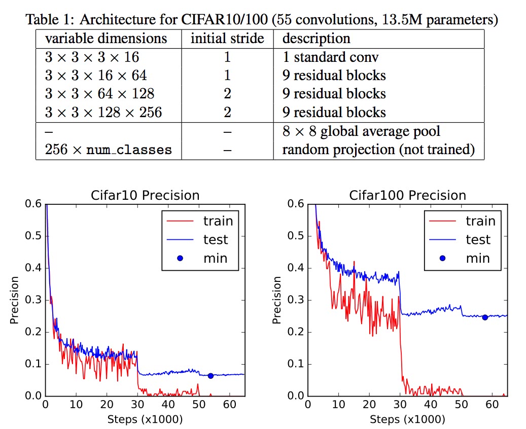
Convergence plots of best model for CIFAR10 (left) and CIFAR (100) right.
Working on CIFAR10 and CIFAR100, the authors tweaked a standard ResNet architecture in Tensorflow to have constant size $c$ of convolution, no batch norm and smaller weight initialization.8 Several features stand out:
- The last layer is a fixed random projection. Therefore all parameters are in the convolutioms.
- Lack of batchnorm or other regularizers seemed not to lead to serious overfitting, even though the model had $\sim 13.6 \times 10^6$ parameters.
- Both problems where tackled with the same networks and the convolutions where of constant size.
Finally, results on ImageNet were not as bright, though the authors seem confident that this is due to lack of tuning of hyperparameters and learning rate. It would be interesting to find out how true this is and how much harder this tuning becomes by having discarded regularization techniques like dropout or additional data processing.
Extensions
For further work in the non-linear case (which as of this writing is reported to be work in progress) where the model is no longer to be assumed correct but instead only (mild) regularity assumptions are made, be sure to check out Bartlett’s talk Representational and optimization properties of Deep Residual Networks .
- See Batch normalization: accelerating deep network training by reducing internal covariate shift . ⇧
- See Deep Residual Learning for image recognition . ⇧
- For extensions to the non-linear setting see Representational and optimization properties of Deep Residual Networks . Note that even though in principle the network can be flattened to only one linear map by taking the product of all $A_{i}$ with no loss in its representational capacity, a great cost in efficiency can be incurred in doing so, see Why does deep and cheap learning work so well? (§G). The dynamics of optimization also are affected by the stacking of purely linear layers, see e.g. Exact solutions to the nonlinear dynamics of learning in deep linear neural networks, (2013) . ⇧
- Essentially, the theorem states that there exists a constant $\gamma$ depending on the largest and smallest singular values of $R$ such that there exists a global minimum $A^{\star}$ of the population risk fulfilling $\underset{1 \leqslant i \leqslant l}{\max} | A^{\star}_{i} | \leqslant \frac{1}{l} (4 \pi + 3 \gamma)$ whenever the number of layers $l \geqslant 3 \gamma$. ⇧
- Equation (2.3) of the paper provides a lower bound on the gradient which does guarantee convergence under the assumption that iterates don’t jump out of the domain of interest. See the reference in the paper. ⇧
- This is a deliberately simpler setup than the original ResNets with two ReLU activations and two instances of batch normalization. See Identity Mappings in Deep Residual Networks, (2016) . ⇧
- An interesting point is the use of the Johsonn-Lindestrauss lemma to ensure that an initial random projection of input data onto $\mathbb{R}^k$ by the first layer does not violate the condition that it remains separated, with high probability. ⇧
- Gaussian with $\sigma \sim (k^{- 2} c^{- 1})$ instead of $\sigma \sim (k^{- 1} c^{- 1 / 2})$. For more on proper initialisation see e.g. On the importance of initialization and momentum in deep learning, (2013) . ⇧