tl;dr: Normalization to zero mean and unit variance of layer outputs in a deep model vastly improves learning rates and yields improvements in generalization performance. Approximating the full sample statistics by mini-batch ones is effective and computationally manageable. You should be doing it too.
Covariate shift and whitening
For any procedure learning a function $f$ from random data $X \sim \mathbb{P}_{X}$ it is essential that the distribution itself does not vary along the learning process.1 When it does, one says that there is covariate shift, a phenomenon which one clearly wishes to avoid or mitigate.2 One possibility is to “fix” the first two moments of $\mathbb{P}_{X}$ by whitening: the transformation on the full sample data
\[ \boldsymbol{x} \mapsto \hat{\Sigma}^{- 1 / 2} (\boldsymbol{x}- \hat{\boldsymbol{\mu}}) \]
subtracting the sample average and multiplying by the inverse covariance matrix centers the data around 0 and decorrelates features to have unit variance and vanishing covariance (assuming positive definiteness). This is long known to yield faster convergence rates.3
Consider now a general feed forward neural network
\[ f = f_{L} \circ \cdots \circ f_{1} \]
with arbitrary (non linear) layers $f_{l} = f_{l} (\cdot ; \theta _{l})$. Updates to the layer parameters $\theta _{1}, \ldots, \theta _{L}$ during training will alter the mean, variance and other statistics of the activations of each layer $f_{l}$ acting as input for layer $f_{l + 1}$, that is: the distributions $f_{l} (\tilde{X} ; \theta _{l})$ will shift, or, in other words, the subnetwork experiences covariate shift. One says that the (full) network suffers internal covariate shift.
So even if we do the usual normalization of the training data (the input to $f_{1}$) and initialise all the weights to have 0 mean and unit variance, the distributions $f_{1} (X), (f_{2} \circ f_{1}) (X), \ldots$ will shift as training progresses. This is bad enough for learning itself, but it will have further negative impact in networks using saturating activations like sigmoids, since it will tend to move them into saturating regimes where learning stops.
In today’s paper, the authors propose a method of approximately whitening each layer with reduced computational cost.
Batch normalization
In order to improve training one would like to whiten all activations by interspersing $L - 1$ additional layers
\[ g_{l} (x, \theta _{l}) = \hat{\Sigma}_{l}^{- 1 / 2} (x - \hat{\mu}_{l}), \]
where $\hat{\mu}_{l}$ and $\hat{\Sigma}_{l}$ are the full sample mean and covariance, taking into account the network parameters $\theta _{l}$ (up to layer $l$) distorting the training data. In the case of a linear network, the transformation $f_{l} (x) = Wx + b$ maps the random input $X_{l}$ to $X_{l + 1}$ by shifting its mean by $b$ and scaling the covariance $C_{X_l}$ to $C_{X_{l + 1}} = WC_{X_l} W^{\top}$. This transformation only affects the first two moments, so that it can be undone by whitening. When one adds nonlinear effects, it is hoped that this first order approximation will be enough to keep the distribution of $X_{l + 1}$ under control.
It is clear that computing these quantities is utterly impractical: they change for each layer after each parameter update and depend on the full training data. Note however that the “obvious” simplification of ignoring the effect of $\theta _{l}$ and taking statistics only over the training data, instead of over the intermediate activations can lead to layers not updating their parameters even for nonzero gradients.4 For this reason the authors propose two simplifications:
- Normalize each component $x^{(k)}$ of an activation independently \[ \operatorname{Norm} (x)^{(k)} = \frac{x^{(k)} - \hat{\mu}^{(k)}}{\hat{\sigma}^{(k)}} . \] This avoids computing covariance matrices and still improves convergence even if there are cross-correlations among features.
- Compute statistics $\mu _{l, B}$ and $\sigma _{l, B}$ at each layer $l$ for SGD mini-batches $B = \lbrace x_{B_1}, \ldots, x_{B_n} \rbrace $ instead of over the full sample (these are rough approximations to the “true” statistics $\mu _{l}, \sigma _{l}$ at a layer with fixed parameters).
In order to have a functioning method, there is an important addition to make: because simply normalizing activations changes the regime in which the next layer operates,5 two parameters $\gamma _{l}, \beta _{l} \in \mathbb{R}^d$ are added to allow for linear scaling of the normalized activations, in principle enabling the undoing of the normalization.6
The final batch normalization layer looks like
\[ \operatorname{BN}_{l} (x^{(k)}) = \frac{x^{(k)} - \hat{\mu}_{l, B}^{(k)}}{\sqrt{\hat{\sigma}_{l, B}^{(k)} + \varepsilon}} \gamma _{l}^{(k)} + \beta _{l}^{(k)}, \]
where $\hat{\mu}^{(k)}_{l, B}$ is the sample mean of the $k$-th component of the activations in minibatch $B$, $\hat{\sigma}_{l, B}^{(k)}$ is the sample variance of the same component, and $\varepsilon > 0$ avoids divisions by too small numbers. It is important to stress the fact that we are not computing statistics over the training data but over the activations computed for a given minibatch, which includes the effect of all relevant network parameters.
Test time
At each training step $t$ we have normalized each layer using “local” batch mean and variances, which again, depended on the current parameters $\theta _{l}^t$ of the network. In the limit $\theta^t_{l} \rightarrow \theta _{l}^{\star}$ for some (locally) optimal $\theta^{\star}_{l}$, we have some fixed population mean and variance of the activations at this layer, $X_{l} = f_{l} (X_{l - 1} ; \theta^{\star}_{l})$ which, intuitively, we should use at test time. To estimate these quantities, we use can use the pertinent full-sample statistics, rather than mini-batch, $\hat{\mu}, \hat{\sigma}$ for layer activations:7
\[ \operatorname{BN} (x^{(k)}) = \frac{\gamma^{(k)}}{\sqrt{\hat{\sigma}^{(k)} + \varepsilon}} x^{(k)} + \left( \beta^{(k)} - \frac{\gamma^{(k)} \hat{\mu}^{(k)}}{\sqrt{\hat{\sigma}^{(k)} + \varepsilon}} \right) . \]
However computing full covariance matrices is typically out of the question so we approximate these by averaging different $\hat{\mu}_{B}, \hat{\sigma}_{B}$ over multiple minibatches, and in practice this is usually done with a moving average during training. It is clear that all this requires some rigorous developments in order to be fully satisfactory…
Application, learning rates and regularization
The first application is to convolutional nets, in particular a modified Inception8 network for ImageNet classification. Here normalization is performed before the nonlinearity, because as explained above, the linear layer only alters the first order moments of its input so normalization of first moments makes more sense there. This has the additional benefit of dispensing with the bias parameters since they are subsumed into $\beta$. There are further details to be taken into account for convnets, see the paper for details.
As already mentioned, BN is conjectured to be advantageous for optimization because
it prevents small changes to the parameters from amplifying into larger and suboptimal changes in activations in gradients; for instance, it prevents the training from getting stuck in the saturated regimes of nonlinearities.
A further conjecture, based on a heuristic argument assuming Gaussianity, is that it
may lead the layer Jacobians to have singular values close to 1, which is known to be beneficial for training.9
Finally, it was experimentally observed that some sort of regularization is performed by BN, to the point that Dropout10 could be entirely omitted in some examples. Again, some rigorous work is required here.
In practice
It is noted that BN alone does not fully exploit its potential. One needs to adapt the architecture and optimization by (details in the paper):
- Increasing the learning rate and its rate of decay.
- Removing dropout (or reducing the dropout probability) and reducing the $L^2$ weight regularization.
- Removing Local Response Normalization.
Furthermore, improving the quality shuffling of training examples for minibatches (by preventing samples to repeatedly be chosen together) and decreasing the intensity of transformations in augmented data proved beneficial. The overall results are impressive (best performance at ImageNet at the time):
Merely adding Batch Normalization to a state-of-the-art image classification model yields a substantial speedup in training. [With the modifications mentioned] we reach the previous state of the art with only a small fraction of training steps – and then beat the state of the art in single-network image classification. Furthermore, by combining multiple models trained with Batch Normalization, we perform better than the best known system on ImageNet, by a significant margin.
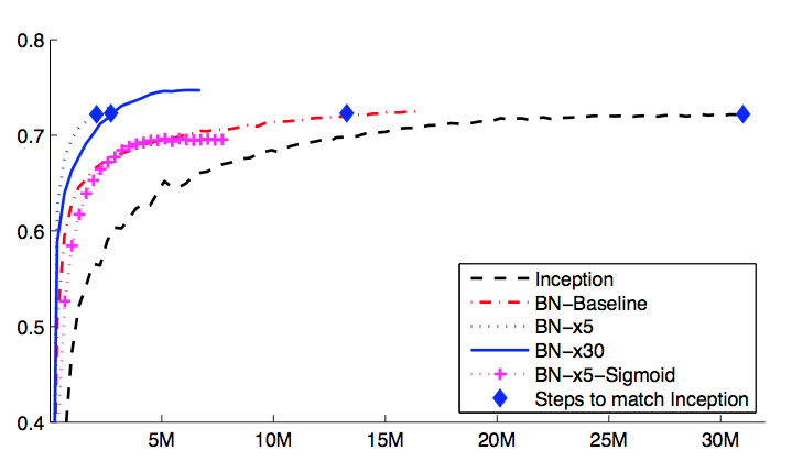
Single crop validation accuracy of Inception and its batch-normalized variants, vs. the number of training steps.
Some recent developments
Since the introduction of BN, several related techniques have been developed. Two prominent ones are:
- Layer normalization: normalize the output of each unit in layer $l$ by the mean and variance of all other outputs given just one example.11
- Weight normalization: activations are normalized by the norm of the weights.12 Faster but still performant.
Twists on BN include:
- Diminishing Batch Normalization: Convergence Analysis of Batch Normalization for Deep Neural Nets, Yintai Ma, Diego Klabjan
- Recurrent Batch Normalization,Tim Cooijmans, Nicolas Ballas, César Laurent, Çağlar Gülçehre, Aaron Courville.
- To be updated…
- Think e.g. of any PAC generalization bounds: even in these worst-case estimates, the sampling distribution, albeit arbitrary, has to be fixed. ⇧
- Improving predictive inference under covariate shift by weighting the log-likelihood function, (2000) introduces the term covariate shift for the difference between the distribution of the training data and the test data, the first being typically heavily conditioned by the sampling method and the second being the “true” population distribution. The authors of the current paper extend its meaning to a continuous “shifting under the feet” of the training distribution. ⇧
- Efficient BackProp, (1998) already discussed using mean normalization in neural networks, as well as many of its properties, together with whitening. ⇧
- Details in §2 of the paper. ⇧
- E.g. by limiting the input to a sigmoid to be $\mathcal{N} (0, 1)$ it will roughly operate in its linear regime around 0. ⇧
- $\gamma_l$ and $\beta_l$ will be learnt along all other parameters $\theta$ whereas the precise batch mean $\mu _{l, B}$ and variance $\sigma _{l, B}$ vary with each training step since they depend on the parameters $\theta$ of each layer and the minibatch. If they were good estimators of some “true” population moments $\mu _{l}, \sigma _{l}$ then we could say that the batch normalization layer could become an identity if the optimization required it, but it is not clear what this true distribution would be since it changes at each point in parameter space. Also, even if we only consider $\mu _{l}, \sigma _{l}$ at local minima for the energy, where the network is supposed to converge, there can be many of them… ⇧
- Note that we rewrite the operation as $ax + b$ to point out that all quantities but $x$ are constant at test time. ⇧
- Going deeper with convolutions, (2015) . ⇧
- Exact solutions to the nonlinear dynamics of learning in deep linear neural networks, (2013) . ⇧
- Improving neural networks by preventing co-adaptation of feature detectors . ⇧
- Layer Normalization, (2016) . ⇧
- Weight Normalization: A Simple Reparameterization to Accelerate Training of Deep Neural Networks, (2016) . ⇧