tl;dr: Deeper models for visual tasks have been proven to greatly outperform shallow ones, but after some point simply adding more layers decreases performance even if the networks are in principle more expressive. Adding skip-connections overcomes these difficulties and vastly improves performance, while keeping the number of parameters under control.
This post is a prequel to previous ones where we went over work studiying the
theoretical properties of Residual Networks, introduced in the current
paper. In
Why does deep and cheap learning work so well?
we learnt that deeper networks are very
good approximators of compositional functions at the expense of energy
landscapes with poorer local optima. Later, in
Identity matters in Deep Learning
we saw that (nonlinear) perturbations of the identity as models are easy to
optimize and are able to learn $r$ classes with $\mathcal{O} (n \log n + r^2)$
parameters, whereas
Representational and optimization properties of Deep Residual Networks
discusses why
Lipschitz functions can (in principle) be very well approximated by resnets.
Changing the hypothesis space to perturbations of the identity for easier
optimization yields vastly improved results. Be sure to check those papers
later.
Deeper is harder
Vanishing gradients used to be a huge issue with deeper networks, which has partly been addressed by normalized initialization and batch normalization.1 However, even if they then converge to some optima, networks with lots of layers show degraded performance. Notably, the problem is not overfitting since they can exhibit poorer training error. But since just stacking more layers can only increase the expressiveness of the class of functions which can be computed, this points to an optimization issue.
The authors suggest then the addition of skip connections among layers with the idea of letting the network preserve relevant features from across layers: in the case that an identity is optimal, it’s just easier to use these connections than to learn weights through the nonlinearities.
Nothing new under the sun
As is (almost) always the case, the idea of propagating residual information is present in many branches of mathematics. The authors mention applications in vector quantization, and more excitingly multigrid methods for PDEs, where each subproblem computes the residual between solutions at each scale. But shortcut connections where also present in the beginnings of neural networks or more recently with highway networks with gated shortcuts (i.e. with trainable additional weights able to shut them off entirely).
Network architecture and implementations
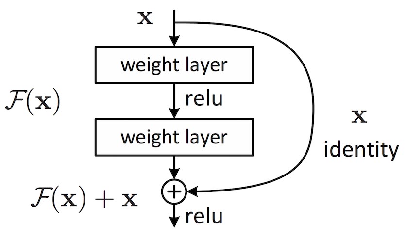
The basic building block of a Residual Network.
Assuming that we augment data in one dimension to include biases into the network’s weight matrices, we can compactly denote the building block of the figure as
\[ \boldsymbol{y}=\mathcal{F} (\boldsymbol{x}, \lbrace W_{i} \rbrace ) +\boldsymbol{x}, \]
where
\[ \mathcal{F} (\boldsymbol{x}, \lbrace W_{i} \rbrace ) = W_{i + 1} \sigma (W_{i} \boldsymbol{x}) . \]
Note that the shortcut $\mathcal{F}+\boldsymbol{x}$ doesn’t add any parameters to the model, which is important not only because of the obvious reason, but also when comparing performance to that of other networks without skip connections.2 Note also that having at least two layers with one nonlinearity is essential for the skip connection to make sense, since otherwise the building block reduces to a linear mapping.
The reasoning behind adding the identity was already mentioned above: the degrading performance of models which are actually more expressive means that they have trouble approximating the identity (since that would be a way of “discarding” unnecessary layers and falling back to the simpler model). It was hoped that by adding the identity this would be mitigated. In fact it effectively changes the hypothesis space to concatenated perturbations of the identity, which are empirically seen to be small because the weights $W_{i}$ are. And we now know thanks to later work that this hypothesis space has very good properties both in terms of approximation ability and optimization properties.
The gist of all the claims made until now can be seen in the very first example of the paper, where the authors consider three models: first a VGG-19 network, second a plain (no residual connections) network of 34 layers inspired by VGG-19’s architecture, and thirdthe second model with skip connections. Recall that the latter maintains the number of parameters wrt. the second model.
The first comparison between 18 and 34 layers display the aforementioned phenomenon of lower performance but no vanishing gradients.
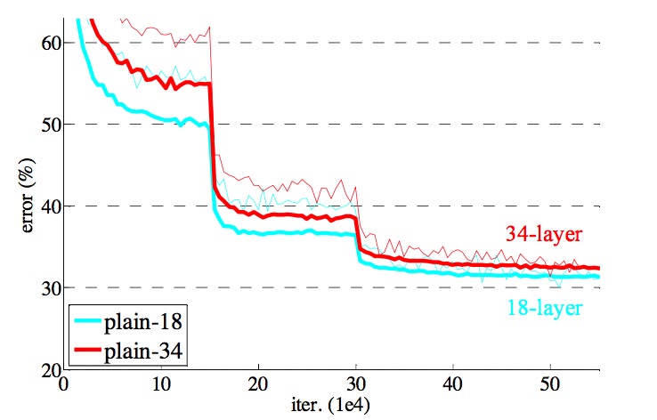
Adding more layers makes optimization harder
The authors conjecture that
this optimization difficulty is unlikely to be caused by vanishing gradients. These plain networks are trained with [Batch Normalization] which ensures forward propagated signals to have non-zero variances. We also verify that the backward propagated gradients exhibit healthy norms with BN. So neither forward nor backward signals vanish.
However, skip connections fix the issue and the interpretation already explained is put forth. Recall again that there is now theoretical work supporting some of the claims.
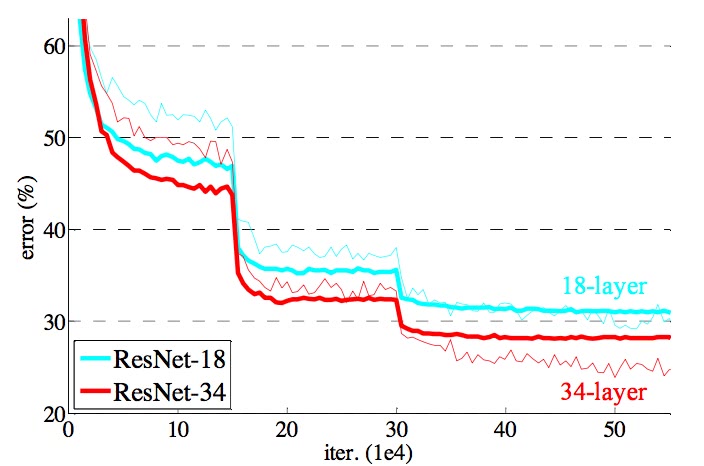
Adding skip connections vastly improves performance
There is also an interesting point with plain networks which are not as deep: adding skip connections to an 18 layer network doesn’t increase performance but it does decrease the time to convergence. Again the optimization landscape is more benign in the new hypothesis space.
Finally the authors report great results with CIFAR-10 and COCO detection and localization which I won’t repeat here because the paper has “all” the details (modulo any actual implementation details ;-).
- Batch normalization: accelerating deep network training by reducing internal covariate shift . ⇧
- One minor modification is required in case $\dim \boldsymbol{x} \neq \dim \mathcal{F}$, namely using some projection matrix to change the dimension: $\boldsymbol{y}=\mathcal{F} (\boldsymbol{x}, \lbrace W_{i} \rbrace ) + W_{s} \boldsymbol{x}$. ⇧