tl;dr: Starting from the intuition that many physical dynamical systems are typically well modeled by first order systems of ODE with governing equations expressed in terms of a few elementary functions, the authors propose a fully connected architecture with multiple non-linearities with the purpose of learning the formulae for these systems of equations. The network effectively performs a kind of hierarchical, non-linear regression with the given nonlinearities as basis functions and is able to learn the governing equations for several examples like a compound pendulum or the forward kinematics of a robotic arm. Crucially, this approach provides good extrapolation performance to unexplored input regimes. For model selection (i.e. hyperparameter choice), competing solutions are scored based both on validation performance and computed model complexity, measured in number of terms in the equations.
Consider the task of designing an adequate model for e.g. the forward kinematics of a robotic arm. For the engineer, the goal is to find some “simple” set of equations with which to compute the state of all joints in phase space given any initial conditions. Designing such a model, potentially exhibiting complex couplings and non-linearities can be a challenging task so one alternative might be to try to learn a statistical model for it. However, standard regression will in many cases prove inadequate because the crucial assumption that the training data sufficiently represent the whole distribution may be violated, e.g. if measurements have not been taken in regimes beyond the normal operating regime of the robot.
The authors propose learning instead the equations for the physical model, i.e. the equations themselves as algebraic expressions composed of coefficients and standard elementary operations like the identity, sums, sines, cosines and binary products.1 By choosing the basis functions to have their support over all of $\mathbb{R}$ (with non negligible mass everywhere) the hope is that extrapolation to conditions not seen during training will be possible.
In par goes an ad-hoc model selection technique: cross-validation is not adequate because it again hinges on the assumption that the whole data distribution is significantly captured with the training data.
The model
The network architecture
Assume that some dynamics $y = \phi (x) + \varepsilon$ are given by an unknown $\phi : \mathbb{R}^n \rightarrow \mathbb{R}^m$ and $\varepsilon$ an $m$-dimensional R.V. with zero mean. The function $\phi$ is assumed to lie in a class $\mathcal{C}$ consisting of compositions of algebraic expressions of elementary functions (sum, product, sine, cosine, …). As usual, the goal is to compute an estimator $\hat{\phi}$ in an adequate hypothesis space $\mathcal{H}$, such that risk wrt. the squared loss $R (\hat{\phi}) =\mathbb{E}_{X, Y} [(\hat{\phi} (X) - Y)^2]$ is minimized. Computation of $\hat{\phi}$ is done by means of minimization of the proxy empirical risk
\[ \hat{R} (\hat{\phi}) := \frac{1}{N} \sum_{i = 1}^N | \hat{\phi} (x_{i}) - y_{i} |^2 . \]
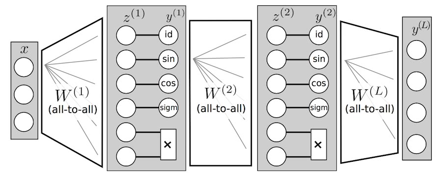
The proposed estimator (EQuation Learner) is similar to hierarchical, non-linear regression with basis functions, in the form of a standard, fully connected, feed forward neural network
\[ \hat{\phi}_{N} (x) = y^{(L)} \circ y^{(L - 1)} \cdots \circ y^{(1)} (x) \]
where the layers $1, \ldots, L - 1$ are the standard composition of a linear mapping $z^{(l)} = W^{(l)} x^{(l - 1)} + b^l$ with a non linearity. And there lies the key contribution:
\[ y^{(l)} (z) = (f_{1} (z_{1}^{(l)}), \ldots, f_{u} (z_{u}^{(l)}), g_{1}^{(l)} (z_{u + 1}, z_{u + 2}), \ldots, g_{v}^{(l)} (z_{u + 2 v - 1}, z_{u + 2 v})) . \]
Here $f_{i}$ are unary maps (identity, $\sin$, $\cos$, $\operatorname{sigm}$) and $g_{j}$ are binary units, currently only multiplication of their inputs, but see below. Note that it is essential to be able to efficiently model multiplication but full multiplication of all entries might lead to polynomials of very high degree, which are uncommon in physical models (but shouldn’t this be sorted out by the optimization / model selection?).
The last layer is simply a linear mapping onto the output vector $y^L$. Each vector of inputs $x \in \mathbb{R}^d$ represents a measurement in phase space. After training, the solution is read from the structure of the network itself: each output $y^L_{k}$ is “followed backward” to obtain one equation, with weights being the coefficients of the operations defined by each unit.
Training and model selection
The objective function is complemented by an $L_{1}$ penalty to induce sparsity (as in the Lasso):
\[ \mathcal{L} (\hat{\phi}_{N}) = \hat{R} (\hat{\phi}_{N}) + \lambda \sum_{j = 1}^L | W^{(l)} |_{1} \]
This is actually done via three-stage optimization: for the first $t_{1}$ steps no penalty is used, then, until some later step $t_{2}$ the lasso term is activated and thereafter deactivated but small weights are clamped to zero and forced to remain there. The goal of this procedure is to let coefficients adjust during the first epochs without being subject to the driving force of the penalty term (which artificially pushes them to lower values), then ensure that lower weights stay there without driving others further down. [Given the ad-hoc nature of this method, it might be interesting to see what happens with some form of best subset selection, like e.g. greedy forward regression.2]
Model selection (choosing how many layers how wide and with how many non-linearities of which kind) proves to be tricky: standard cross-validation requires that sampling from training data be representative of the full data distribution, but precisely one of the desired abilities of this model is that it extrapolate (generalize) beyond its input to data ranges not represented in the training data. Therefore the authors propose a two-goal objective to choose the best architecture among a set $ \lbrace \phi _{k} \rbrace _{k = 1}^K$:
\[ \underset{k = 1, \ldots, K}{\operatorname{argmin}} [(r^v (\phi _{k}))^2 + (r^s (\phi _{k}))^2], \]
where $r^v, r^s : \lbrace \phi _{k} \rbrace _{k = 1} \rightarrow \lbrace 1, \ldots, K \rbrace $
sort (rank) all $K$ models respectively by validation accuracy and and
complexity (measured as the number of units with activation above a given
threshold). This is a way of embedding both measures into a common space ($ \lbrace
1, \ldots, K \rbrace $) for joint optimization.
Because these values might correspond to (possibly poor) local optima subject to the initial values of the parameters, multiple runs are used to “estimate error bars”.
Some ideas
Note: this section does not report results of the paper.
The last fact rises the point of whether one could define population quantities $\rho^v, \rho^s$ over all possible hypothesis spaces $\mathcal{H}$. $\rho^v$ might encode e.g. the minimal risk (i.e. expected loss) $\underset{\hat{\phi} \in \mathcal{H}}{\min} R (\hat{\phi})$, which would be $0$ iff $\mathcal{H} \cap \mathcal{C} \neq \emptyset$, and $\rho^s$ might encode e.g. the capacity of $\mathcal{H}$ or some measure of its complexity. Estimates as to the accuracy of some sample-approximation to these quantities would then be necessary.
An alternative idea to explore could be Bayesian model selection. Basically one postulates some prior over a set of hypothesis spaces $ \lbrace \mathcal{H}_{k} \rbrace _{k = 1}^K$, then computes the posterior of the data given some hypothesis by marginalizing over parameter space $\Omega$:
\[ p (\boldsymbol{t}|\mathcal{H}_{k}) = \int_{\Omega} p (\boldsymbol{t}|W, \mathcal{H}_{k}) p (W|\mathcal{H}_{k}) \mathrm{d} W. \]
This integral will probably not be tractable so it will have to be approximated using MCMC or some other method.
Experiments
It is just easier if you check them in the paper itself. Suffice to say that both pendulum and double pendulum equations were easily learned but also that the hypothesis space $\mathcal{H}$ needs to intersect $\mathcal{C}$ or performance can be quite poor (e.g. if trying to integrate functions without an antiderivative or in an example with a rolling cart attached to a wall through a spring).
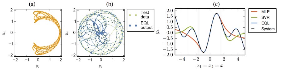
Double pendulum data and extrapolation results for Multi Layer Perceptron, Support Vector Regression and Equation Learner.
Recent work improves on the “bad” examples.
Recent extensions
In a recent (yesterday!) talk at Munich’s Deep Learning Meetup, Martius presented some recent developments around this model, most notably the introduction of division units. Because of the pole at 0, they decided to restrict the domain to positive reals bounded away from zero ($z \geqslant \theta > 0$), while adding a penalty on negative inputs to the unit. The following slide displays their regularized division unit.
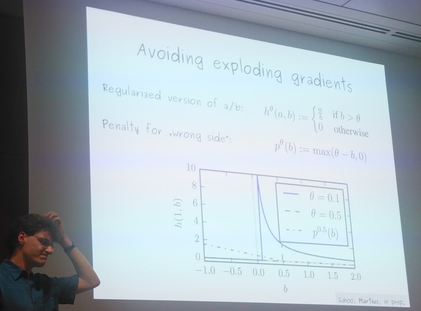
The speaker tries to answer a peculiar question.
Potential optimization issues arising from this regularization clamping the local gradients to 0 were not discussed. It will be very interesting to read about this and any other findings in the forthcoming paper!
Results of course vastly improve in examples involving quotients. This paves the road for further extensions, like arbitrary exponentiation or logarithms.
- Division, square roots and logarithms are explicitly left for later work since their domains of definition are strict subsets of $\mathbb{R}$, thus requiring special handling, e.g. via cut-offs. More on this in the last section. ⇧
- However, see Extended Comparisons of Best Subset Selection, Forward Stepwise Selection, and the Lasso, (2017) . ⇧