tl;dr: Training a network to classify images (with a single label) is modeled as a sequential decision problem where actions are salient locations in the image and tentative labels. The state (full image) is partially observed through a fixed size subimage around each location. The policy takes the full history into account compressed into a hidden vector via an RNN. REINFORCE is used to compute the policy gradient.
Although the paper targets several applications, to fix ideas, say we want to classify images with one label. These can vary in size but the number of parameters of the model will not change. Taking inspiration from how humans process images, the proposed model iteratively selects points in the image and focuses on local patches around them at different resolutions. The problem of choosing the locations and related classification labels is cast as a reinforcement learning problem.
Attention as a sequential decision problem
One begins by fixing one image $x$ and selecting a number $T$ of timesteps. At each timestep $t = 1, \ldots, T$:
- We are in some (observed) state $s_{t} \in \mathcal{S}$: it consists of a location $l_{t}$ in the image (a pair of coordinates), and a corresponding glimpse $x_{t}$ of $x$. This glimpse is a concatenation of multiple subimages of $x$ taken at different resolutions, centered at location $l_{t}$, then resampled to the same size. How many ($k$), at what resolutions ($\rho _{1}, \ldots, \rho _{k}$) and to what fixed size ($w$) they are resampled are all hyperparameters.1 The set of all past states is the history: $s_{1 : t - 1} := \lbrace s_{1}, \ldots, s_{t - 1} \rbrace$.
- We take an action $a_{t} = (l_{t}, y_{t}) \in \mathcal{A}$, with the new location $l_{t}$ in the (same) image $x$ to look at and the current guess $y_{t}$ as to what the label for $x$ is. In the typical way for image classification with neural networks, $y_{t}$ is a vector of “probabilities” coming from a softmax layer. Analogously, the location $l_{t}$ is sampled from a distribution parametrized by the last layer of a network. The actions are taken according to a policy $\pi^t_{\theta} : \mathcal{S}^t \rightarrow \mathcal{P} (\mathcal{A})$, with $S^t = S \times \overset{t - 1}{\cdots} \times S$, and $\mathcal{P} (\mathcal{A})$ the set of all probabilty measures over $\mathcal{A}$. The policy is implemented as a neural network, where $\theta$ represents all internal parameters. The crucial point in the paper is that the network takes the whole history as input, compressed into a hidden state vector, i.e. the policy will be implemented with a recurrent network. Because parameters are shared across all timesteps, we drop the superindex $t$ and denote its output at timestep $t$ by $\pi _{\theta} (a_{t} |s_{1 : t})$.
- We obtain a scalar reward $r_{t} \in \lbrace 0, 1 \rbrace$. Actually, the reward will be 0 at all timesteps but the last ($T$), where it can be either 0 if $y_{T}$ predicts the wrong class or 1 if it is the right one.2
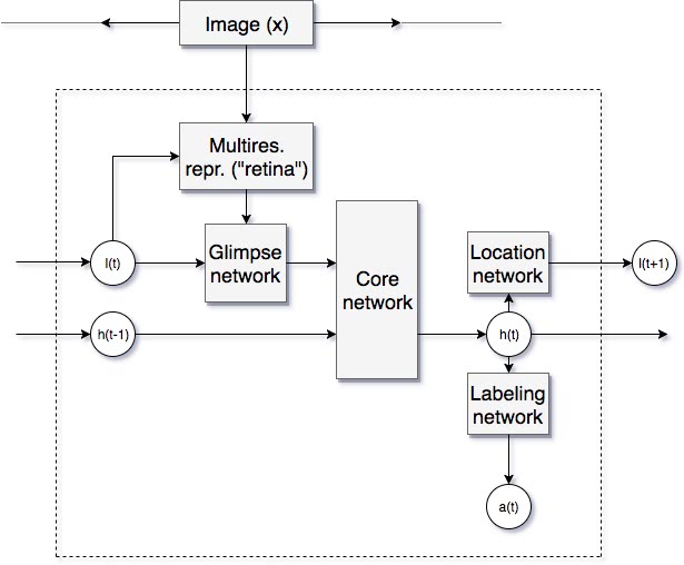
The model at timestep $t$.
Note that the policy $\pi _{\theta} (a_{t} |s_{1 : t})$ has two “heads”, a labeling network $f_{y}$, outputting a probability of the current glimpse belonging to each class and a location network $f_{l}$. Only the output of the latter directly influences the next state. This is important when computing the distribution over trajectories $\tau = (s_{1}, a_{1}, \ldots, s_{T}, a_{T})$ induced by the policy:
\[ p_{\theta} (\tau) := p (s_{1}) \prod_{t = 1}^T \pi _{\theta} (a_{t} \mid s_{t}) p (s_{t + 1} \mid s_{t}, a_{t}) = p (s_{1}) \prod_{t = 1}^T p (l_{t} \mid f_{l} (s_{t} ; \theta)) p (s_{t + 1} \mid s_{t}, l_{t}) . \]
The goal is to maximise the total expected reward
\[ J (\theta) := \mathbb{E}_{\tau \sim p_{\theta} (\tau)} [\sum_{t = 1}^T r (s_{t}, a_{t})] . \]
The algorithm used is basically the policy gradient method with the REINFORCE rule:3
Algorithm 1:
- Initialise $\pi _{\theta}$ with some random set of parameters.
- For $n = 1 \ldots N$, pick some input image $x_{n}$ with label $y_{n}$.
- Sample some random initial location $l_{0}$.
- Run the policy (the recurrent network) $\pi _{\theta}$ for $T$ timesteps, creating new locations $l_{t}$ and labels $y_{t}$. At the end collect the reward$r_{T} \in \lbrace 0, 1 \rbrace$.
- Compute the gradient of the reward $\nabla _{\theta} J (\theta _{n})$.
- Update $\theta _{n + 1} \leftarrow \theta _{n} + \alpha _{n} \nabla _{\theta} J_{\theta} (\theta _{n})$.
The difficulty lies in step $5$ because the reward is an expectation over trajectories whose gradient cannot be analitically computed. One solution is to rewrite the gradient of the expectation as another expectation using a simple but clever substitution:
\[ \nabla _{\theta} J (\theta) = \int \nabla _{\theta} p_{\theta} (\tau) r (\tau) \mathrm{d} \tau = \int p_{\theta} (\tau) \frac{\nabla _{\theta} p_{\theta} (\tau)}{p_{\theta} (\tau)} r (\tau) \mathrm{d} \tau = \int p_{\theta} (\tau) \nabla _{\theta} \log p_{\theta} (\tau) r (\tau) \mathrm{d} \tau, \]
and this is
\[ \nabla _{\theta} J (\theta) =\mathbb{E}_{\tau \sim p_{\theta} (\tau)} [\nabla _{\theta} \log p_{\theta} (\tau) r (\tau)] \]
In order to compute this integral we can now use Monte-Carlo sampling:
\[ \nabla _{\theta} J (\theta) \approx \frac{1}{M} \sum_{m = 1}^M \nabla _{\theta} \log p_{\theta} (\tau_m) r (\tau_m), \]
and after rewriting $\log p_{\theta} (\tau)$ as a sum of logarithms and discarding the terms which do not depend on $\theta$ we obtain:
\[ \nabla _{\theta} J (\theta) \approx \frac{1}{M} \sum_{m = 1}^M \sum_{t = 1}^T \nabla _{\theta} \log \pi _{\theta} (a^m_{t} |s^m_{1 : t}) r^m, \]
where $r^m = r_{T}^m$ is the final reward (recall that in this application $r_{t} = 0$ for all $t < T$). In order to reduce the variance of this estimator it is standard to subtract a baseline estimate $b =\mathbb{E}_{\pi{\theta}} [r{T}]$ of the expected reward, thus arriving at the expression
\[ \nabla _{\theta} J (\theta) \approx \frac{1}{M} \sum_{m = 1}^M \sum_{t = 1}^T \nabla _{\theta} \log \pi _{\theta} (a^m_{t} |s^m_{1 : t}) (r^m - b) . \]
There is a vast literature on the Monte-Carlo approximation for policy gradients, as well as techniques for variance reduction.4
Hybrid learning
Because in classification problems the labels are known at training time, one can provide the network with a better signal than just the reward at the end of all the process. In this case the authors
optimize the cross entropy loss to train the [labeling] network $f_{y}$ and backpropagate the gradients through the core and glimpse networks. The location network $f_{l}$ is always trained with REINFORCE.
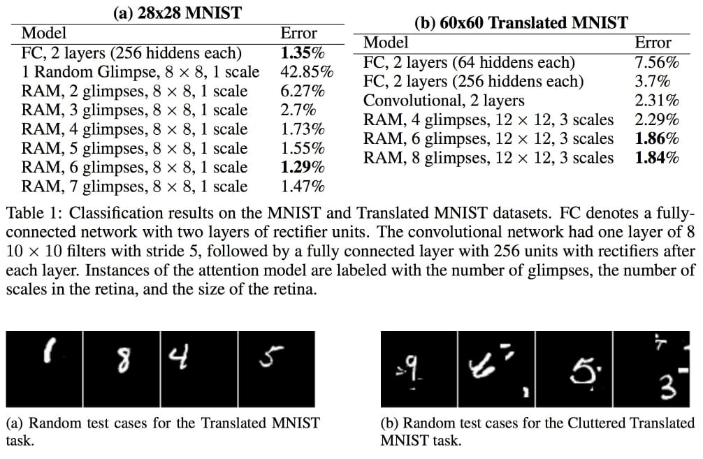
Results for image classification
An image is worth a thousand words:
- It would be nice to try letting a CNN capture the relevant features for us, instead of fixing the resolutions. I’m sure this has been tried since 2014. ⇧
- I wonder: wouldn’t it make more sense to let $r_{t} \in [0, 1]$ instead using the cross entropy to the 1-hot vector encoding the correct class? ⇧
- See e.g. Reinforcement Learning: An Introduction, (2018) , §13.3. ⇧
- Again, see Reinforcement Learning: An Introduction, (2018) . ⇧