Today’s post is about another great talk given at the Simons Institute for the Theory of Computing in the context of their currently ongoing series Computational Challenges in Machine Learning.
Part 1: Variational, Hamiltonian and Symplectic Perspectives on Acceleration
For convex functions, Nesterov accelerated gradient descent method attains the optimal rate of $\mathcal{O} (1 / k^2)$.1
\begin{equation}
\label{eq:nesterov}\tag{1} \left \lbrace \begin{array}{lll}
y_{k + 1} & = & x_{k} - \beta \nabla f (x_{k})\\
x_{k + 1} & = & (1 - \lambda _{k}) y_{k + 1} + \lambda _{k} y_{k} .
\end{array}\right.
\end{equation}
Note that this is not actually gradient descent since the momentum will make the trajectory deviate from the “steepest slope” at some point.
Gradient descent is a discretization of gradient flow:
\[ \dot{X}_{t} = - \nabla f (X_{t}) . \]
Nesterov’s method is the discretisation of the ODE2
\begin{equation} \label{eq:su-boyd-candes-ode}\tag{2} \ddot{X}_{t} + \frac{3}{t} \dot{X}_{t} + \nabla f (X_{t}) = 0. \end{equation}
Question 1: These ODEs are obtained by taking continuous time limits. Is there a deeper generative mechanism?
The Lagrangian point of view
For a target function $f$ to optimize, define the Bregman Lagrangian
\begin{equation} \label{eq:lagrangian}\tag{3} \mathcal{L} (x, \dot{x}, t) = \mathrm{e}^{\gamma _{t} + \alpha _{t}} (D_{h} (x + \mathrm{e}^{- \alpha _{t}} \dot{x}, x) - \mathrm{e}^{\beta _{t}} f (x)), \end{equation}
where the exponentials and parameters provide degrees of freedom for later fine-tuning, $D_{h}$ is the Bregman divergence
\[ D_{h} (y, x) = h (y) - h (x) - \langle \nabla h (x), y - x \rangle \]
taken between $x$ and $x$ plus some (scaled) velocity $\dot{x}$, and $h$ is the convex distance-generating function for $D_{h}$. Note that if one takes $h (x) = x^2 / 2$, then $D_{h} (\ldots) = \frac{1}{2} | \dot{x} |^2$ is the kinetic energy so we always interpret this term as such and the second one $- \mathrm{e}^{\beta _{t}} f (x)$ as the potential energy whose well we are going down. The choice of $h$ will depend on the geometry of the problem, i.e. on the space where minimization happens.
The scaling functions $\alpha _{t}, \beta _{t}, \gamma _{t}$ are in fact fixed by certain ideal scaling conditions reducing them to one effective degree of freedom. This constraint has been designed to obtain the desired rates below, but the whole parameter space has not been explored.
The Euler-Lagrange equation for the minimization over paths with starting point $X_{0}$
\begin{equation} \label{eq:minimization-paths}\tag{4} \min _{X} \int \mathcal{L} (X_{t}, \dot{X}_{t}, t) \mathrm{d} t \end{equation}
is called the non-homogenous master ODE:3
\begin{equation} \label{eq:master-ode}\tag{5} \ddot{X}_{t} + (\mathrm{e}^{\alpha _{t}} - \dot{\alpha}_{t}) \dot{X}_{t} + \mathrm{e}^{2 \alpha _{t} + \beta _{t}} [\nabla^2 h (X_{t} + \mathrm{e}^{- \alpha _{t}} \dot{X}_{t})]^{- 1} \nabla f (X_{t}) = 0. \end{equation}
The claim is that
this is going to generate (essentially) all known accelerated gradient methods in continuous time.
The first result is a rate in continuous time:4
Theorem 2: Under ideal scaling, the E-L equation (5) has convergence rate \[ f (X_{t}) - f (x^{\star}) \leqslant \mathcal{O} (\mathrm{e}^{- \beta _{t}}) \] to the optimum $x^{\star}$.
In discrete time, for general smooth convex problems it is known that this rate cannot be attained, although for uniformly convex ones it can. So, what is going on?
Suppose we had $\beta _{t} = p \log t + \log C$, then $\alpha _{t}, \gamma _{t}$ are fixed by the ideal scaling relations and (5) has $\mathcal{O} (\mathrm{e}^{- \beta _{t}}) =\mathcal{O} (1 / t^p)$. The master ODE is now
\[ \ddot{X}_{t} + \frac{p + 1}{t} \dot{X}_{t} + Cp^2 t^{p - 2} \left[ \nabla^2 h \left( X_{t} + \dfrac{t}{p} \dot{X}_{t} \right) \right]^{- 1} \nabla f (X_{t}) = 0. \]
With $p = 2$ one obtains (2). Plugging different values of $p$ yields other methods (like accelerated cubic-regularized Newton’s method for $p = 3$). The interesting point is that $\mathcal{L}$ is a covariant operator: a reparametrization of time (in particular a change in $p$) does not change the solution path.
Under these assumptions we have an optimal way to optimze: there is a particular path and acceleration is just changing the speed at which you move along it.
Note that this is not a property of gradient flow: reparametrization changes the path. In general it will be different from the one obtained from (4).
Question: (audience, “Nahdi”?) Is it possible to introduce new parameters into the master ODE (or change the current ones) to interpolate in some way between Nesterov-like methods and gradient flow?
The answer is that indeed, the whole range of $\alpha _{t}, \beta _{t}, \gamma _{t}$ has not been exhausted and “we could recover other algorithms by exploring [it]”.
Discretizing the E-L equation (1)
(While preserving stability and the convergence rate). The first thing one thinks of is to reduce the 2nd order equation to a 1st order system and apply e.g. an Euler scheme to obtain an algorithm. The problem is that the method is not stable! (and it lost the rate)
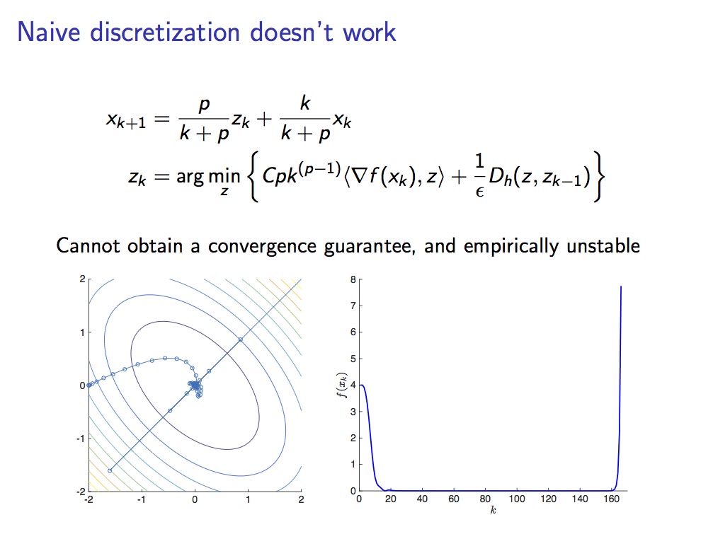
Instability of conventional methods for the master ODE.
Then one can try Runge-Kutta or whatever: they all lose stability and the rate. Jordan’s group saw two approaches for solving this problem: “reverse-engineer the Nesterov estimate sequence technique” interpreting it as a discretization method or use symplectic integration (see below). For the first one it is possible to recover oracle rates by increasing the assumptions on $f$:
Theorem 3: Assume $h$ is uniformly convex and introduce an auxiliary sequence $y_{k}$ into the “naive” Euler discretization. Assuming higher regularity on $f (y_{k})$: \[ f (y_{k}) - f (x^{\star}) \leqslant \mathcal{O} \left( \frac{1}{\varepsilon k^p} \right) . \]
But one typically does not want to have to assume these additional conditions on $\nabla f$ (Lipschitz $p - 1$ derivatives).
Discretizing the E-L equation (2): symplectic integration
Symplectic integration is a numerical integration technique which conserves quantities like energy and momentum in a (time-dependent) Hamiltonian framework.5 By taking the Legendre transform (a.k.a. Fenchel conjugate) of the velocity and time one obtains momentum and energy respectively and can write a Hamiltionian which basically mimics the Lagrangian we had (it has the form (3) modulo constants and signs). Then one solves Hamilton’s equations in phase space with a discretization which looks at and conserves a certain local volume tensor / differential form along the path of integration.
Why is this interesting in our setting? The discretization seen for the Lagrangian formulation suffers from high sensitivity to step size and a momentum build-up which hurts performance near the optimum. The Hamiltonian perspective produces equivalent equations whose symplectic integration should alleviate these issues and achieve faster rates without further assumptions : conservation of momentum seems to be the key.
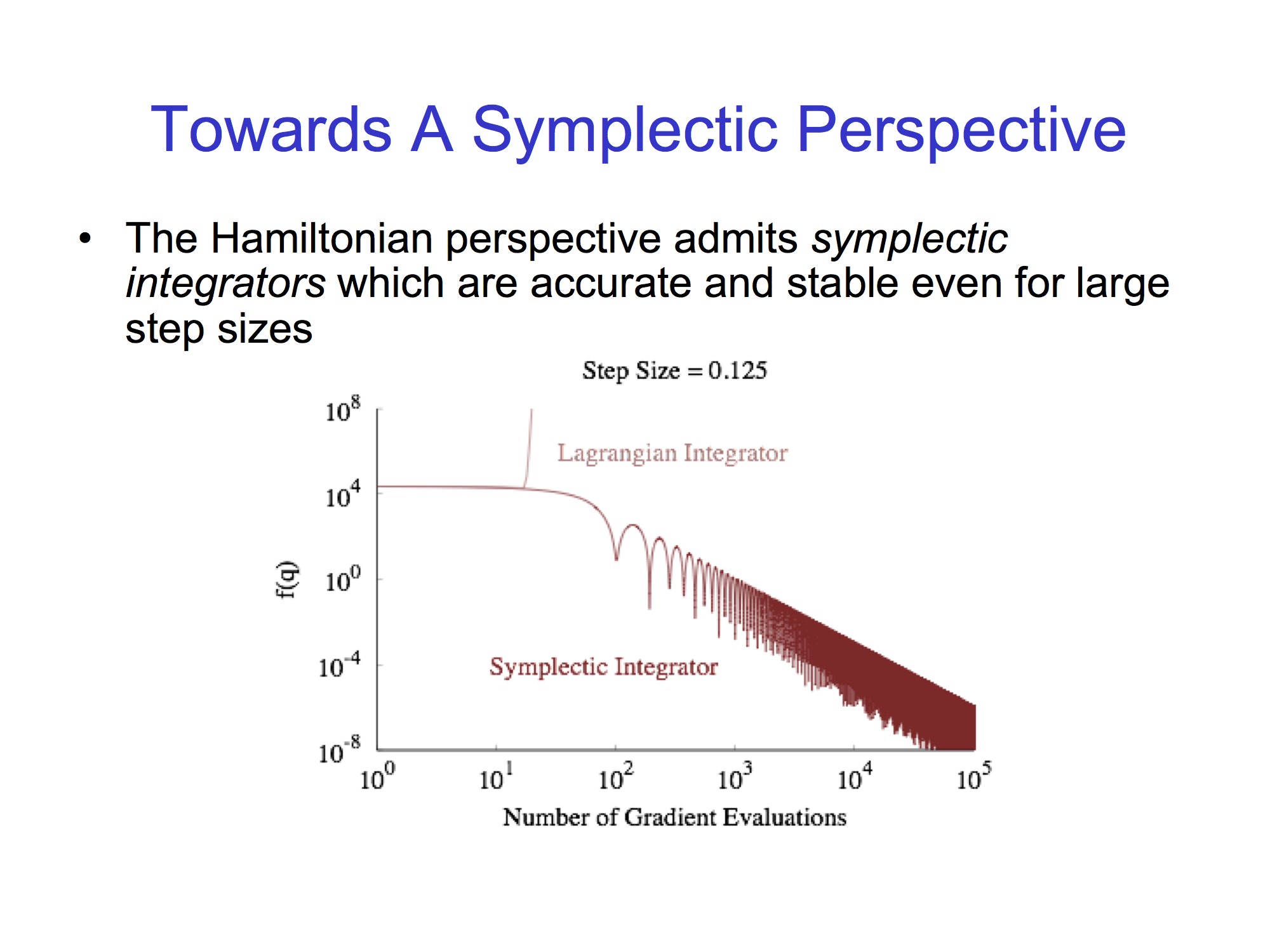
Comparing Lagrangian and Symplectic integrators.
Ongoing / future / related work
Two possible venues for exploration are:
- Non-convex setting: the framework described can be applied as well.
- Stochastic equations: there will probably also exist an “optimal way to diffuse” in SDEs derived from some Focker-Planck type equation.
- Since we are in a smooth convex setting, there is a global minimum: if you know it, then you trivially attain it in one step. Besides this useless case, if one has higher order derivatives, then higher order methods provide faster convergence rates and so on. For this reason one needs to restrict the definition of optimality in some sense. The concept of an oracle was introduced with this purpose: An oracle is an entity which “answers” questions of an optimization scheme about the function to be optimized (e.g. what is the value of $\nabla f$ at $x_{k}$?), within the model of the problem (i.e. it represents the things known to the method). This leads to the definition of the class of smooth first order methods as those which only have access to gradient infromation and produce iterates of the form $x_{k} \in x_{0} +\operatorname{span} \lbrace \nabla f (x_{0}), \ldots, \nabla f (x_{k - 1}) \rbrace $. It is under this restriction that Nesterov’s gradient descent achieves the optimal rate of $\mathcal{O} (1 / k^2)$. See e.g. Introductory Lectures on Convex Optimization - A Basic Course, (2004) , Chapter 1 for more on oracles and §2.1.2 for the previous statements, originally proved in A method of solving a convex programming problem with convergence rate O (1/k2), (1983) . ⇧
- A differential equation for modeling Nesterov’s accelerated gradient method: Theory and insights, (2016) write a finite differences equation for (1), take limit as the stepsize goes to zero and find the continuous equation. ⇧
- Note that this has roughly the form of a damped oscillator with the additional “geometric term” involving the Hessian of the distance generating function, evaluated at “$X$ plus velocity” (yielding the acceleration). ⇧
- The proof is a one-liner choosing and adequate Lyapunov function. Note however that (as explained later) by reparametrizing the equation one can change the rate, so this is not groundbreaking news for the continuous setting. It is the passage to the discrete setting and the conditions under which the rate can or cannot be achieved that matter. ⇧
- Symplectic intregrators are also used in the hybrid Montecarlo method, an MCMC technique where the transition between states is governed by Hamiltonian dynamics. ⇧