tl;dr: dropout (of features) for GLMs is a noising procedure equivalent to Tykhonov regularization. A first order approximation of the regularizer actually scales the parameters with the Fisher information matrix, adapting the objective function to the dataset, independently of the labels. This makes dropout useful in the context of semi-supervised learning: regularizers can be adapted to the unlabeled data yielding better generalization. For logistic regression the adaption amounts to favoring features on which the estimator is confident.
For shallow architectures, there were already some (stated) results on the averaging properties of dropout.1 This was later extended to multiple layers with sigmoid units: simple weighting of outputs in the forward pass computes an approximation of the expectation of the ensemble.2 Today’s paper predates this work and focuses still on shallow networks, albeit within the wider scope of Generalized Linear Models.
Since these are shallow models, dropout is performed on the inputs and it can be compared to other methods of input perturbation like additive Gaussian noise.
There are 3 main contributions in this paper:
- A dropout regularizer for a GLM is (up to first order) equivalent to a classical Tykhonov regularizer with $L^2$-norm, with a specific scaling. Crucially, this scaling depends on the data but not on the labels and makes the regularization adaptive.
- Incorporating this regularization into a rewriting of SGD as the repeated solution of regularized linear problems leads to an update similar to AdaGrad.3 A connection between the goals of both is established.
- In the case of logistic regression the dropout regularizer is shown to favour confident predictions, regardless of the label (in the sense that it penalizes less those weights corresponding to features on which the predicted probability is far from $1 / 2$). Therefore it makes sense to apply it to semi-supervised problems computing an extra term over unlabeled data.
(Feature-) Dropout is weighted $L^2$-regularization
Consider any Generalized Linear Model with parameters $\beta$, inputs $x \in \mathbb{R}^d$ and outputs $y \in Y$, i.e.4
\[ p (y|x, \beta) = h (y) \mathrm{e}^{yx \beta - A (x \beta)}, \]
and negative log likelihood as the loss. For one training sample $(x, y)$: $l (\beta ; x, y) = - \log p (y|x, \beta)$. Now choose some noise vector $\xi \in \mathbb{R}^d$ with i.i.d. entries with zero mean and replace $x \mapsto \tilde{x}$ where $\tilde{x}$ has been noised with $\xi$ in some way we specify later. A couple of computations show that the empirical loss on the (full) noised data $\tilde{\boldsymbol{x}} = (\tilde{x}_{1}, \ldots, \tilde{x}_{n}),\boldsymbol{y}= (y_{1}, \ldots, y_{n})$ is the loss on the original data plus a new term:
\[ \hat{L} (\tilde{\boldsymbol{x}}, \boldsymbol{y}, \beta) = \hat{L} (\boldsymbol{x}, \boldsymbol{y}, \beta) + R (\beta), \]
which is the noising regularizer
\begin{equation} \label{eq:noising-regularizer}\tag{1} R (\beta) := \sum_{i = 1}^n \mathbb{E}_{\xi} [A (\tilde{x}_{i} \beta)] - A (x_{i} \beta) . \end{equation}
$R (\beta)$ has two key features:
- It does not depend on the labels: this will allow for its use in unsupervised setting.
- It is adapted to the training data.
But how exactly “adapted”? Definition (1) is quite impenetrable as is, even after plugging in a specific $A$. Assuming we can do a Taylor expansion of $A$ around $x \beta$ one obtains5
\[ \mathbb{E}_{\xi} [A (\tilde{x} \beta)] - A (x \beta) \approx \tfrac{1}{2} A” (x \beta) \operatorname{Var}_{\xi} [\tilde{x} \beta] \]
and substituting into (1) the (approximate) quadratic noising regularizer:
\begin{equation} \label{eq:quadratic-noising-regularizer}\tag{2} R^q (\beta) := \sum_{i = 1}^n \tfrac{1}{2} A” (x \beta) \operatorname{Var}_{\xi} [\tilde{x} \beta] . \end{equation}
Note that (2) is in general non-convex. When questioned by a reviewer about this fact, the authors respond
Although our objective is not formally convex, we have not encountered any major difficulties in fitting it for datasets where n is reasonably large (say on the order of hundreds). When working with LBFGS, multiple restarts with random parameter values give almost identical results. The fact that we have never really had to struggle with local minimas suggests that there is something interesting going on here in terms of convexity.
We can now fix the noising method and look at its variance to gain insight into what $R^q$ does, and hopefully, by extension $R$.6 The authors consider:
- Additive gaussian noise: $\tilde{x} = x + \xi$ with $\xi _{i}$ i.i.d. spherical Gaussians $\mathcal{N} (0, \sigma^2 \operatorname{Id}_{d})$.
- Dropout noise: fix $\delta \in (0, 1)$ to build a (scaled) binary mask $\xi$ with i.i.d entries $\operatorname{Bernoulli} (1 - \delta)$ and set $\tilde{x} = x \odot \xi / (1 - \delta)$ to cancel some of the inputs with probability $\delta$.7
Notice that in both cases $\mathbb{E}_{\xi} [\tilde{x}] = x$ and the expectation of the Taylor expansion of $A$ yields (2) (that’s the reason for the scaling factor $\delta$). After performing the necessary computations, and assuming the design matrix has been normalized to $\Sigma _{i j} x^2_{i j} = 1$, the authors obtain the following neat table:
The first row holds by definition. The first column recovers known results8 and adds the fact that dropout (after scaling) on linear regression is ridge regression. It’s the box who tells a more interesting story. First we note that the key matrix $V (\beta) \in \mathbb{R}^{n \times n}$ is diagonal with entries $V (\beta)_{i i} = A” (x_{i} \beta)$.
Additive noising for logistic regression penalizes more strongly uncertain predictions ($p_{i} \approx 0.5$). For arbitrary GLMs, $R^q$ is just multiplied by a constant.
Dropout in logistic regression has the same feature as additive noise plus selective exclusion of features: given a training sample $x_{i}$, $\beta _{j}$ is not penalized if $x_{i j} = 0$. In particular $p_{i} (1 - p_{i})$ and $\beta _{j}$ may both be large if the cross-term $x_{i j}^2$ is small. This means that
(…) dropout regularization should be better than $L^2$-regularization for learning weights for features that are rare (i.e., often 0) but highly discriminative, because dropout effectively does not penalize $j$ over observations for which $x_{i j} = 0$.
And
dropout rewards those features that are rare and positively co-adapted with other features in a way that enables the model to make confident predictions whenever the feature of interest is active.
In the more general case the insight comes from the fact that
\[ \tfrac{1}{n} X^{\top} V (\beta^{\star}) X = \tfrac{1}{n} \sum_{i = 1}^n \nabla^2 l (\beta^{\star} ; x_{i}, y_{i}) \]
is an estimator of the Fisher information matrix $\mathcal{I}$. Therefore if we write $\beta^{\top} \operatorname{diag} (X^{\top} V (\beta) X) \beta = \beta^{\top}D \beta = | D^{1 / 2} \beta |_{2}^2 = | \tilde{\beta} |_{2}^2$ we see that dropout is applying an $L^2$ penalty after normalizing with an approximation of $\operatorname{diag} (\mathcal{I})^{- 1 / 2}$.
The Fisher information is linked to the shape of the level surfaces of $l (\beta)$ around $\beta^{\star}$. If $\mathcal{I}$ were a multiple of the identity matrix, then these level surfaces would be perfectly spherical around $\beta^{\star}$.
By normalizing, the feature space is deformed into a shape where “the features have been balanced out”.9 The authors provide a very nice picture for intuition:
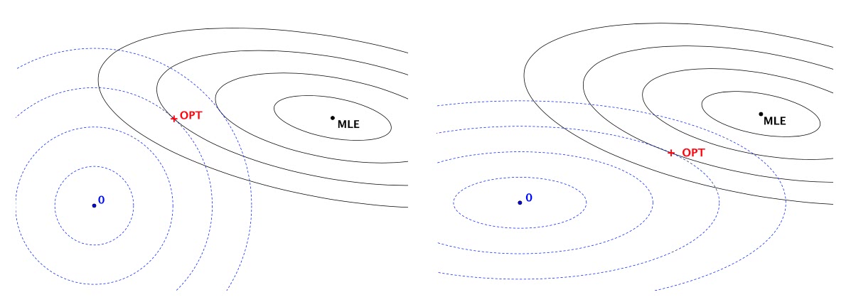
Comparison of two $L^2$ regularizers.
(page 11 in the Appendix)In both cases, the black solid ellipses are level surfaces of the likelihood and the blue dashed curves are level surfaces of the regularizer; the optimum of the regularized objective is denoted by OPT. The left panel shows a classic spherical $L^2$ regular izer $| \beta |_{2}^2$, whereas the right panel has an $L^2$ regularizer $\beta^{\top} \operatorname{diag}(\mathcal{I}) \beta$ that has been adapted to the shape of the likelihood ($\mathcal{I}$ is the Fisher information matrix). The second regularizer is still aligned with the axes, but the relative importance of each axis is now scaled using the curvature of the likelihood function. As argued [above], dropout training is comparable to the setup depicted in the right panel.
Relation to AdaGrad
By rewriting standard SGD into an iterative solution of linear $L^2$-penalized problems
\[ \hat{\beta}_{t + 1} = \operatorname{argmin}_{\beta} \left \lbrace l (\hat{\beta}_{t} ; x_{t}, y_{t}) + \nabla l (\hat{\beta}_{t}) (\beta - \hat{\beta}_{t}) + \frac{1}{2 \eta _{t}} | \beta - \hat{\beta}_{t} |_{2}^2 \right \rbrace \]
and substituting the dropout penalty for the penalty in this formulation, one obtains the update rule
\[ \hat{\beta}_{t + 1} =\operatorname{argmin}_{\beta} \left \lbrace l (\hat{\beta}_{t} ; x_{t}, y_{t}) + g_{t} (\beta - \hat{\beta}_{t}) + R^q (\beta - \hat{\beta}_{t} ; \hat{\beta}_{t}) \right \rbrace \]
with the centered quadratic dropout penalty, similarly to the entry in Table 1:
\[ R^q (\beta - \hat{\beta}_{t} ; \hat{\beta}_{t}) = (\beta - \hat{\beta}_{t})^{\top} \operatorname{diag} (X^{\top} V (\hat{\beta}_{t}) X) (\beta - \hat{\beta}_{t}) . \]
This is effectively solving the problem of SGD has learning weights for “rare but highly discriminative features”, by using the update
\[ \hat{\beta}_{t + 1} = \hat{\beta}_{t} - \eta _{t} A_{t}^{- 1} \nabla l (\hat{\beta}_{t}) . \]
AdaGrad10 uses $A_{t} =\operatorname{diag} (\nabla^{\top} l (\hat{\beta}_{t}) \nabla l(\hat{\beta}_{t}))^{- 1 / 2}$, warping the gradient by some sort of intrinsic metric, whereas dropout uses its estimate of the Fisher information.11 However, in the limit $\hat{\beta}_{t} \rightarrow \beta^{\star}$ for GLMs the expectations of both matrices are equal to $\mathcal{I}$, meaning that the SGD updates when using feature dropout in GLMs are “converging” in some sense to AdaGrad updates.
Semi-supervised tasks
As we said above, the dropout regularizer is shown to change the loss function with the Fisher information matrix in a way that focuses on weights relevant for discriminative features, without recourse to the labels $y_{i}$. Therefore in a semi-supervised context, we can use unlabeled data to improve the regularizer:
\[ R_{\ast} (\beta) := \frac{n}{n + \alpha m} \left( R (\beta) + \alpha R_{\text{unlabeled}} (\beta) \right), \]
where $n$ is the size of the labeled dataset, $m$ that of the unlabeled one and $\alpha$ a “discount factor” for the latter which is a hyperparameter. Unlike other semi-supervised approaches relying on generative models, the authors’ approach
is based on a different intuition: we’d like to set weights to make confident predictions on unlabeled data as well as the labeled data, an intuition shared by entropy regularization [24] and transductive SVMs [25].
- See Improving neural networks by preventing co-adaptation of feature detectors . ⇧
- See Understanding Dropout , The Dropout Learning Algorithm, (2014) . ⇧
- See Adaptive Subgradient Methods for Online Learning and Stochastic Optimization, (2011) . ⇧
- Recall that in a GLM one uses a so-called link function $h$ to relate a linear predictor $x \beta$ with the posterior $p (y|x)$ by means of the relationship $\mathbb{E} [y|x] = h^{- 1} (x \beta)$. In our notation, $h = A’$. To fix ideas think of logistic regression, where $p (y|x) = (1 + \mathrm{e}^{- x \beta})^{- 1}$. In this case we assume $y \in \lbrace 0, 1 \rbrace $, the log likelihood is $p (\boldsymbol{y}|\boldsymbol{x}) = \prod_{i} p_{i}^{y_{i}} (1 -p_{i})^{1 - y_{i}}$, with $p_{i} := (1 + \mathrm{e}^{- x_{i} \beta})^{- 1}$ and the negative log likelihood is the cross entropy loss: $\log p (y|x) = - \sum_{i} y_{i} \log p_{i} + (1 - y_{i}) \log (1 -p_{i})$. ⇧
- Indeed $A (\tilde{x} \beta) - A (x \beta) = A’ (x \beta) (\tilde{x} \beta - x \beta)+ \frac{1}{2} A” (x \beta) (\tilde{x} \beta - x \beta)^2 + \text{h.o.t.}$ and taking expectations: $\mathbb{E}_{\xi} [A (\tilde{x} \beta)] - A (x \beta) = A’ (x \beta) (\mathbb{E} [\tilde{x} \beta] - x \beta) + \frac{1}{2} A” (x \beta)\mathbb{E} (\tilde{x} \beta - x \beta)^2 + \text{h.o.t}$. ⇧
- There is a handwavy discussion in the paper on the error $| R - R^q |$ which is not worth discussing here. Suffice to say: it works “well” in practice. ⇧
- Here $\odot$ stands for the entrywise or Hadamard product. ⇧
- See Training with noise is equivalent to Tikhonov regularization for more on additive noise leading to ridge regression. ⇧
- Notice that we could use any quadratic form to redefine the norm in which weights are measured. There are surely many other interesting possibilities! ⇧
- See Adaptive Subgradient Methods for Online Learning and Stochastic Optimization, (2011) . ⇧
- This looks like a nice connection to second order methods: warp the update step with information on the target function or warp feature space with information on the data to “improve” it (very handwavily put…) ⇧