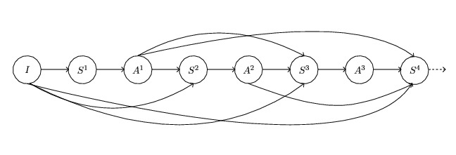
The authors set to study the “averaging” properties of dropout in a quantitative manner in the context of fully connected, feed forward networks understood as DAGs. In particular, architectures other than sequential are included, cf. Figure 1. In the linear case with no activations, the output of some layer $h$ (no dropout yet) is:

$$ S^h_i = \sum_{l < h} \sum_j w^{h l}_{i j} S^l_j . $$

And if activations are included:

\begin{equation} O^h_i = A (S_i^h) = A \left( \sum_{l < h} \sum_j w^{h l}_{i j} O^l_j \right), \label{dag-network} \tag{1} \end{equation}

with $O^0_i = I_i$. The authors consider only sigmoid and exponential activation functions $A$.

Recall that dropout consists of randomly disabling (i.e. setting to 0) some fraction of the outputs at each layer.¹ This means that for some fixed input, randomness is introduced in the model by the dropout scheme. The authors only explicitly consider i.i.d. “Bernoulli gating variables” $\delta^l_j$ (at layer $l$, output $j$) which disable outputs with probability $p^l_j$ (but mention that the results extend to other distributions):

\begin{equation} O^h_i = \sigma (S_i^h) = \sigma \left( \sum_{l < h} \sum_j w^{h l}_{i j} \delta^l_j O^l_j \right) . \label{eq:dropout-bernoulli} \tag{2} \end{equation}

Note that probabilities and expectations are therefore always over the set of all possible subnetworks, not over the input data.

The key result is the following estimate on the expected value of an output, using the Normalized Weighted Geometric Mean:

\begin{equation} \mathbb{E} (O^h_i) \overset{(\dagger)}{\approx} \text{NWGM} (O^h_i) \overset{(\ast)}{=} A_i^h (\mathbb{E} [S_i^h]) \overset{(\triangle)}{=} A_i^h (\sum_{l < h} \sum_j w^{h l}_{i j} p^l_j \mathbb{E} (O^l_j)), \label{eq:main-estimate} \tag{3} \end{equation}

where the NWGM is defined as the quotient $\text{NWGM} (x) = G (x) / (G (x) - G’ (x))$ where $G (x) = \prod_i x_i^{p_i}$ is the weighted geometric mean of the $x_i$ with weights $p_i$, and $G’ (x) = \prod_i (1 - x_i)^{p_i}$ the weighted geometric mean of their complements.

In (3), $(\ast)$ holds exactly only for sigmoid and constant functions (p. 2) and $(\triangle)$ follows from independence. The approximation $(\dagger)$ (Section 4) is shown to be exact for linear layers and to hold to first order in general. An interesting observation is that the Ky Fan inequality tells us:

$$ G \leqslant \frac{G}{G + G’} \leqslant E \text{, if } 0 < O_i \leqslant 0.5 \text{ for all } i, $$

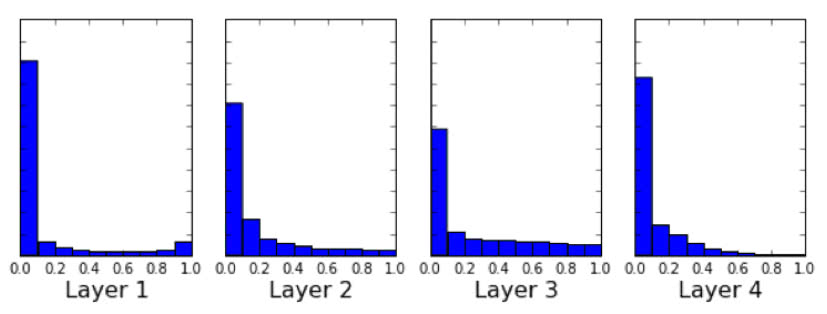
and empirical tests show that:

In every hidden layer of a dropout trained network, the distribution of neuron activations $O^∗$ is sparse and not symmetric.

This seems to indicate that the NWGM is in practice a good approximation when using sigmoidal units. Note however that the bound in eq. (22) $| \mathbb{E}- \text{NWGM} | \leqslant 2\mathbb{E} (1 -\mathbb{E}) | 1 - 2\mathbb{E} |$ seems rather rough, as Figure 3 shows:

Analysis of gradient descent: Using dropout means optimizing simultaneously over the training set and the whole set of possible networks. Therefore, two quantities of interest are the ensemble error

$$ E_{\text{ENS}} = \frac{1}{2} \sum_i (t_i - O^i_{\text{ENS}})^2$$

and the dropout error

$$ E_D = \frac{1}{2} \sum_i (t_i - O^i_D)^2 . $$

In the case of a single linear unit (!) it is show that:

$$ \mathbb{E} (\nabla E_D) = \nabla (E_{\text{ENS}} + R_{\text{ENS}}) $$

with the usual $l^2$ regularizer (here for just one training sample $I$)

$$ R_{\text{ENS}} = \frac{1}{2} \sum_j w^2_j I_j^2 \text{Var} (\delta_j) . $$

So in expectation, the gradient of the dropout network is the gradient of a regularized ensemble. Observe that:

Dropout provides immediately the magnitude of the regularization term which is adaptively scaled by the inputs and by the variance of the dropout variables. Note that $p_i=0.5$ is the value that provides the highest level of regularization.

Analogously, for a single sigmoid unit: the expected value of the gradient of the dropout network is approximately the gradient of a regularized ensemble network:

$$ \mathbb{E} (\nabla E_D) \approx \nabla E_{\text{ENS}} + \lambda \sigma’ (S_{\text{ENS}}) w_j I_j^2 \text{Var} (\delta_j) . $$

These results are extended to deeper networks in: The Dropout Learning Algorithm, Baldi, P. , Sadowski, P. (2014)

Simulations: the validity of the bounds is tested using Monte Carlo approximations to the ensemble distribution. It is shown in several examples how dropout favours the sparsity of activations and “increases the consistency of layers” after dropout layers.