tl;dr: this paper introduced an activation function for deep convolutional networks which specifically benefits from regularization with dropout¹ and still has a universal approximation property for continuous functions. It is hypothesized that, analogously to ReLUs, the locally linear character of these units makes the averaging of the dropout ensemble more accurate than with fully non-linear units. Although sparsity of representation is lost wrt. ReLUs, backpropagation of errors is improved by not clamping to 0, resulting in significant performance gains.

Recall the intuition behind dropout: for each training batch, it masks out around 50% of the units, thus training a different model / network of the $2^N$ possible (albeit all having shared parameters), where $N$ is the total number of units in the network. Consequently it is benefficial to use higher learning rates in order to make each one of the models profit as much as possible from the batch it sees. But then at test time one needs either to sample from the whole ensemble again by using dropout or to use some averaging trick. We recently² saw that simply scaling the outputs actually approximates the expected output of an ensemble of shallow, toy networks, but at the time there was little rigorous work on the averaging properties of dropout.³

Explicitly designing models to minimize this approximation error may thus enhance dropout’s performance

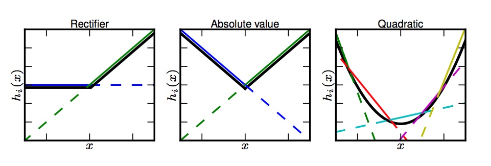
Hence the idea of maxout: define a new activation function

\begin{equation} \label{eq:def-maxout} h_i (x) = \underset{j \in [k]}{\max} z_{i j}, x \in \mathbb{R}^d, i \in [m] \end{equation}

where $z \in \mathbb{R}^{m \times k}$ is a collection of $k$ affine maps computed as $z_{i j} = x_l W_{l i j} + b_{i j}$ (summation convention) and $W \in \mathbb{R}^{d \times m \times k}, b \in \mathbb{R}^{m \times k}$ are to be learned. So

In a convolutional network, a maxout feature map can be constructed by taking the maximum across $k$ affine feature maps (i.e., pool across channels, in addition [to] spatial locations).⁴

The key observation here with respect to the approximation properties of maxout networks is the fact that since we are taking the max over a family of affine functions, the graph of the resulting function is a convex set, so with maxout units we are producing piecewise linear (PWL) convex functions:

Because we have

Theorem: Any continuous PWL function can be expressed as a difference of two convex PWL functions [of the form (1)]. The proof is given in General constructive representations for continuous piecewise-linear functions, Wang, S. (2004) .

and because PWL functions approximate continuous ones over compact sets by Stone-Weierstrass, it immediately follows that maxout networks are universal approximators. Of course we can’t say anything about rates of convergence, so this statement, though necessary is not exactly powerful.

It is important to note that because they don’t clamp to 0 like ReLUs do,

The representation [maxout units produce] is not sparse at all (…), though the gradient is highly sparse and dropout will artificially sparsify the effective representation during training.

After extensive cross-validated benchmarking where maxout basically outperforms everyone (see the paper for the now not-so-much-state-of-the-art results) at MNIST, CIFAR10, CIFAR100 and SVHN we come to the question of why it performs so much better than ReLUs.

The first aspect is the number of parameters required: maxout performs better with more filters, while ReLUs with more outputs and the same number of filters ). But since cross-channel pooling typically reduces the amount of parameters for the next layer

the size of the state and the number of parameters must be about $k$ times higher for rectifiers to obtain generalization performance approaching that of maxout.

The second aspect is the good interplay with dropout and model averaging. The fundamental observation now is that

dropout training encourages maxout units to have large linear regions around inputs that appear in the training data.

The intuitive idea is that these large regions make it relatively rare that the maximal filter selected changes when the dropout mask does, and given the conjecture (?) that

dropout does exact model averaging in deeper architectures provided that they are locally linear among the space of inputs to each layer that are visited by applying different dropout masks,

it seems plausible that maxout units improve the ability to optimize when using dropout. However, this is also true of ReLUs and indeed

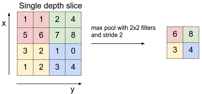
The only difference between maxout and max pooling over a set of rectified linear units is that maxout does not include a 0 in the max.

The experiments in §8.1 show however that this clamping impedes the optimization process and indicate why maxout units are easier to optimize than ReLUs. This observation was already done by Deep sparse rectifier neural networks : dropout induces sparsity (saturation at 0 for ReLUs) and backprop stops at saturated units, but

Maxout does not suffer from this problem because gradient always flows through every maxout unit –even when a maxout unit is 0, this 0 is a function of the parameters and may be adjusted.

It is interesting to see how the experiments where designed in order to single out characteristics of the optimization:

1. Train a small network on a large dataset. Lack of parameters will make it hard to fit the training set.

2. Train a deep and narrow model on MNIST. Vanishing gradients (both for numerical reasons and because of the clamping to 0 blocking gradients) will make optimization hard.⁵

3. Train two-layer MLPs with 1200 filters per layer and 5-channel max-pooling: adding a constant 0 deactivates units and degrades performance over simply taking the max.

A final noteworthy test to keep in mind is keeping track of the variances of the activations. Maxout networks enjoyed much higher variance at lower layers than ReLU networks: an indication of the vanishing gradient problem.